Engineers are often faced with the task of optimizing models that have variables that have tolerances. Ideally, an optimized design should be insensitive to the allowable tolerances of all of its variables. As such, designers need to know the sensitivity of each design objective to each variable. The Objective Sensitivity Analysis option of Multi-Objective-OPT will provide the designer with this important information. To illustrate this option’s capability, we have chosen a modified version of MATLAB's "Sombrero" function:

 

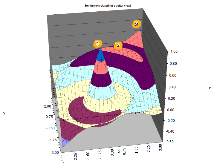
Note that the function contains three local optimums. Local Optimum 1 is the tip of the 'hat' and represents a very sensitive optimum due to the fact that it rapidly falls from the peak.  Local Optimum 2 is also not likely to be the best solution because its gradient is steep as it approaches the 'corner' of the design space. However, Local Optimum 3 may be the best solution because it is not sensitive to changes at its location within the design space. It is easy to use Multi-Objective-OPT's Objective Sensitivity Analysis option to investigate the sensitivity of every local optimum within the design space. First, let's look at the model in Excel and our optimization specification:



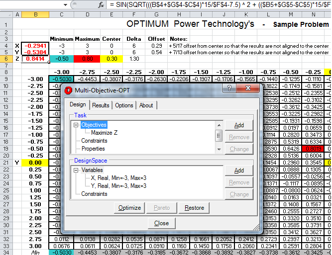
Note that Z (B6) is the function that creates the 3D plot above using the variables X (B4) and Y (B5). In Multi-Objective-OPT, it is very easy to specify the Objective to Maximize Z by altering the variables X and Y as seen in the Multi-Objective-OPT user interface window.  Next we specify the optimization parameters:



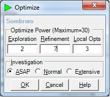
We have selected 3 Local Opts so that we can compare their Z value Objective sensitivities to both their X and Y variables. The default Exploration Power of 0, will only create 1 Local Optimum, so the first Iteration was run with Exploration Power=1. It produced only 2 Local Opts, so the Exploration Power was set to 2. The 2,7,3 ASAP optimization yielded the following results:



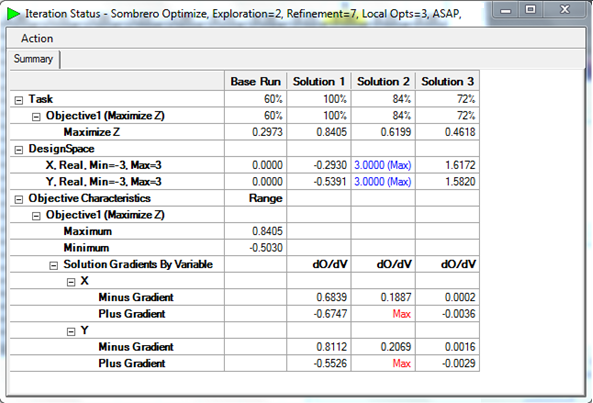
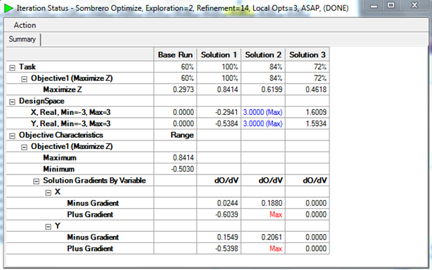
These three solutions are the same three discussed above in the 3D plot. Multi-Objective-OPT has rated Solution 1 (the tip of the 'hat') as the best solution (100%) while the other two are rated 84% and 72% respectively, below it. Objective Sensitivity Analysis shows the Objective’s Gradients by variable in both the Minus and Plus direction. It is easy to see that Solution 3 is the only one with small Gradients in both directions.

Further optimization iterations were performed increasing the Refinement power from 7 to 14 to confirm that this Gradient Analysis was correct. Note that Solution 2 has hit "max" values of the design space so it's sensitivity remains undetermined and is likely not a good candidate. Solution 1's Plus Gradient has not decreased much from the previous run. However, Solution 3's plus and minus gradients are 0, indicating that this solution is insensitive to tolerances. See below:



This rigorous analysis of a complex design space is made easy with Multi-Objective-OPT’s Objective Sensitivity Analysis Option.